REQUEST COMPLIMENTARY SQLS*PLUS LICENCE
Pandas instead of SQL: Working with data in a new way

Previously, SQL as a tool was enough for research analysis: quick data search and preliminary report on data.
Nowadays, data come in different forms and do not always refer to them as “relational databases”. They can be CSV files, plain text, Parquet, HDF5, and many others. This is where the Pandas library can help you.
What is Pandas?
Pandas is a library in the Python language, created for data analysis and processing. It has an open-source code and is supported by Anaconda developers. This library is well suited for structured (tabular) data. More information can be found in the documentation. Pandas allow you to generate data queries and much more.
SQL is a declarative language. It allows you to declare everything in such a way that a query is similar to a normal sentence in English. The syntax of Pandas is very different from SQL. Here you apply operations to a dataset and chain them together for conversion and modification.
SQL parsing
An SQL query consists of several keywords. Between these words are added data characteristics that you want to see. An example of a query framework without specifics:
SELECT... FROM... WHERE...
GROUP BY...
ORDER BY...
LIMIT... OFFSET...
There are other expressions, but these are the most basic. To translate expressions into Pandas, you need to load the data first:
import pandas as pd
airports = pd.read_csv('data/airports.csv')
airport_freq = pd.read_csv('data/airport-frequencies.csv')
runways = pd.read_csv('data/runways.csv')
You can download this data here.
SELECT, WHERE, DISTINCT, LIMIT
Below are several variants of expressions with the SELECT operator. Unnecessary results are cut off with LIMIT and filtered out with WHERE. DISTINCT is used to remove duplicate results.
| SQL | Pandas |
|---|---|
select * from airports | airports |
select * from airports limit 3 | airports.head(3) |
select id from airports where ident = 'KLAX' | airports[airports.ident == 'KLAX'].id |
select distinct type from airport | airports.type.unique() |
SELECT with multiple conditions
Several selection conditions are combined using the operand &. If you only want a subset of some columns from a table, this subset is used in another pair of square brackets.
| SQL | Pandas |
|---|---|
select * from airports where iso_region = 'US-CA' and type = 'seaplane_base' | airports[(airports.iso_region == 'US-CA') & (airports.type == 'seaplane_base')] |
select ident, name, municipality from airports where iso_region = 'US-CA' and type = 'large_airport' | airports[(airports.iso_region == 'US-CA') & (airports.type == 'large_airport')][['ident', 'name', 'municipality']] |
ORDER BY
By default, Pandas will sort the data in ascending order. For reverse sorting use the expression ascending=False.
| SQL | Pandas |
|---|---|
select * from airport_freq where airport_ident = 'KLAX' order by type | airport_freq[airport_freq.airport_ident == 'KLAX'].sort_values('type') |
select * from airport_freq where airport_ident = 'KLAX' order by type desc | airport_freq[airport_freq.airport_ident == 'KLAX'].sort_values('type', ascending=False) |
IN and NOT IN
To filter not a single value but whole lists, there is an IN condition. In Pandas, the .isin() operator works exactly the same way. To override any condition, use ~ (tilde).
| SQL | Pandas |
|---|---|
select * from airports where type in ('heliport', 'balloonport') | airports[airports.type.isin(['heliport', 'balloonport'])] |
select * from airports where type not in ('heliport', 'balloonport') | airports[~airports.type.isin(['heliport', 'balloonport'])] |
GROUP BY, COUNT, ORDER BY
Grouping is performed using the .groupby() operator. There is a small difference between COUNT semantics in SQL and Pandas. In Pandas .count() will return non-null/NaN values. To get a result like in SQL, use .size().
| SQL | Pandas |
|---|---|
select iso_country, type, count(*) from airports group by iso_country, type order by iso_country, type | airports.groupby(['iso_country', 'type']).size() |
select iso_country, type, count(*) from airports group by iso_country, type order by iso_country, count(*) desc | airports.groupby(['iso_country', 'type']).size().to_frame('size').reset_index().sort_values(['iso_country', 'size'], ascending=[True, False])
|
Below is a grouping by several fields. By default, Pandas sorts by the same field list, so in the first example, there is no need for .sort_values(). If you want to use different fields for sorting or DESC instead of ASC as in the second example, you need to specify the selection explicitly:
| SQL | Pandas |
|---|---|
select iso_country, type, count(*) from airports group by iso_country, type order by iso_country, type | airports.groupby(['iso_country', 'type']).size() |
select iso_country, type, count(*) from airports group by iso_country, type order by iso_country, count(*) desc | airports.groupby(['iso_country', 'type']).size().to_frame('size').reset_index().sort_values(['iso_country', 'size'], ascending=[True, False])
|
The use of .to_frame() and .reset_index() is determined by sorting by a specific field (size). This field must be part of the DataFrame type. After grouping in Pandas, the result is another type called GroupByObject. Therefore you need to convert it back to DataFrame. With .reset_index(), the line numbering for the data frame is restarted.
HAVING
In SQL, you can additionally filter grouped data using the HAVING condition. In Pandas, you can use .filter() and provide the Python function (or lambda expression), which will return True if a group of data is to be included in the result.
| SQL | Pandas |
|---|---|
select type, count(*) from airports where iso_country = 'US' group by type having count(*) > 1000 order by count(*) desc | airports[airports.iso_country == 'US'].groupby('type').filter(lambda g: len(g) > 1000).groupby('type').size().sort_values(ascending=False) |
The first N records
Let’s say some preliminary queries have been made and there is now a data frame named by_country that contains the number of airports in each country:
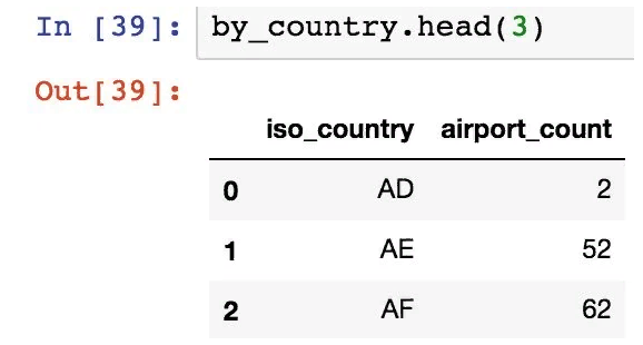
In the following example, let’s organize airport_count data and select only the first 10 countries with the largest number of airports. The second example is a more complex case, where we select the “next 10” after the first 10 entries:
| SQL | Pandas |
|---|---|
select iso_country from by_country order by size desc limit 10 | by_country.nlargest(10, columns='airport_count') |
select iso_country from by_country order by size desc limit 10 offset 10 | by_country.nlargest(20, columns='airport_count').tail(10) |
Aggregate functions: MIN, MAX, MEAN
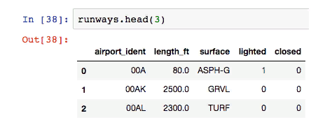
Considering the data frame above (runway data), let’s calculate the minimum, maximum, and average runway length.
| SQL | Pandas |
|---|---|
select max(length_ft), min(length_ft), mean(length_ft), median(length_ft) from runways | runways.agg({'length_ft': ['min', 'max', 'mean', 'median']}) |
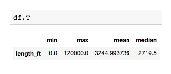
Note that with an SQL query, the data is a column. But in Pandas, the data is represented by rows.
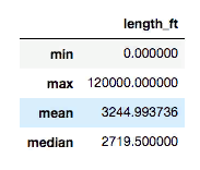
The data frame can be easily transposed with .T to get the columns.
JOIN
Use .merge() to attach data frames to Pandas. You need to specify which columns to join (left_on and right_on) and the connection type: inner (default), left (corresponds to LEFT OUTER in SQL), right (RIGHT OUTER in SQL) or outer (FULL OUTER in SQL).
| SQL | Pandas |
|---|---|
select airport_ident, type, description, frequency_mhz from airport_freq join airports on airport_freq.airport_ref = airports.id where airports.ident = 'KLAX' | airport_freq.merge(airports[airports.ident == 'KLAX'][['id']], left_on='airport_ref', right_on='id', how='inner')[['airport_ident', 'type', 'description', 'frequency_mhz']] |
UNION ALL and UNION
pd.concat() is the UNION ALL equivalent in SQL.
| SQL | Pandas |
|---|---|
select name, municipality from airports where ident = 'KLAX' union all select name, municipality from airports where ident = 'KLGB' | pd.concat([airports[airports.ident == 'KLAX'][['name', 'municipality']], airports[airports.ident == 'KLGB'][['name', 'municipality']]]) |
The UNION equivalent (deduplication) is .drop_duplicates().
INSERT
So far, only sampling has been performed, but data can be changed during the preliminary analysis. In Pandas, there is no INSERT equivalent in SQL to add the required data. Instead, you should create a new data frame containing new records and then combine the two frames.
| SQL | Pandas |
|---|---|
create table heroes (id integer, name text); | df1 = pd.DataFrame({'id': [1, 2], 'name': ['Harry Potter', 'Ron Weasley']}) |
insert into heroes values (1, 'Harry Potter'); | df2 = pd.DataFrame({'id': [3], 'name': ['Hermione Granger']}) |
insert into heroes values (2, 'Ron Weasley'); | |
insert into heroes values (3, 'Hermione Granger'); | pd.concat([df1, df2]).reset_index(drop=True) |
UPDATE
Suppose now you need to fix some incorrect data in the original frame.
| SQL | Pandas |
|---|---|
update airports set home_link = 'http://www.lawa.org/welcomelax.aspx' where ident == 'KLAX' | airports.loc[airports['ident'] == 'KLAX', 'home_link'] = 'http://www.lawa.org/welcomelax.aspx' |
DELETE
The easiest and most convenient way to remove data from a frame in Pandas is to split the frame into rows. Then get line indices and use them in the .drop() method.
| SQL | Pandas |
|---|---|
delete from lax_freq where type = 'MISC' | lax_freq = lax_freq[lax_freq.type != 'MISC'] |
lax_freq.drop(lax_freq[lax_freq.type == 'MISC'].index) |
Variability
By default, most operators in Pandas return a new object. Some operators accept inplace=True, which allows them to work with the original data frame instead of the new one. For example, you can reset the index in a place like this:
df.reset_index(drop=True, inplace=True)
However, the .loc operator (above in the example with UPDATE) simply finds the record indexes to update them, and the values change on the spot. Also, if all values in a column are updated (df[‘url’] = ‘http://google.com’) or a new column is added (df[‘total_cost’] = df[‘price’] * df[‘quantity’]), these data will change in place.
Pandas is more than just a query mechanism. Other transformations can be done with data.
Exporting to many formats
df.to_csv(...) # in csv file
df.to_hdf(...) # in an HDF5 file
df.to_pickle(...) # into the serialized object
df.to_sql(...) # to an SQL database
df.to_excel(...) # to an Excel file
df.to_json(...) # into JSON string
df.to_html(...) # display as an HTML table
df.to_feather(...) # in binary feather format
df.to_latex(...) # in a table environment
df.to_stata(...) # into Stata binary data files
df.to_msgpack(...) # msgpack-object (serialization)
df.to_gbq(...) # in the BigQuery-table (Google)
df.to_string(...) # into console output
df.to_clipboard(...) # in the clipboard that can be inserted into Excel
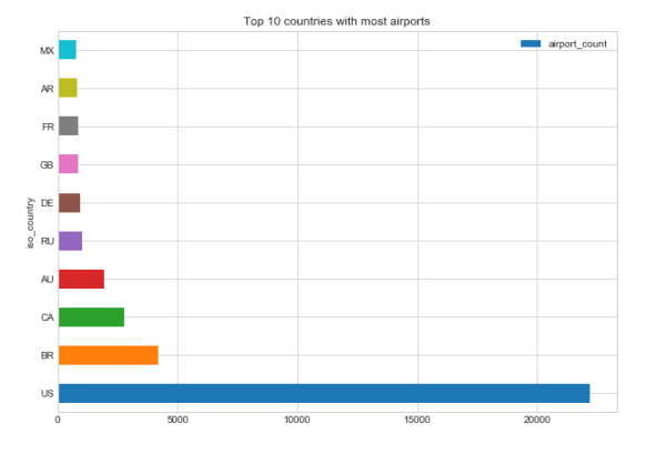
Drawing up charts
top_10.plot(
x='iso_country',
y='airport_count',
kind='barh',
figsize=(10, 7),
title='Top 10 countries with most airports')
We’ll get it:
Opportunity to share your work
The best place to publish Pandas queries, charts, and the like is the Jupyter notebook. Some people (like Jake Vanderplas) even publish whole books there. It is easy to create a new entry in the notebook:
$ pip install jupyter
$ jupyter notebook
After that you can:
- go to the address localhost:8888;
- press “New” and give your notebook a name;
- query and display the data;
- create a GitHub repository and add your notebook (a file with the extension .ipynb).
GitHub has an excellent built-in Jupyter notepad viewer with a Markdown design.
Why Combine Pandas and SQL
MORE NEWS
PreambleNoSql is not a replacement for SQL databases but is a valid alternative for many situations where standard SQL is not the best approach for...
PreambleMongoDB Conditional operators specify a condition to which the value of the document field shall correspond.Comparison Query Operators $eq...
5 Database management trends impacting database administrationIn the realm of database management systems, moreover half (52%) of your competitors feel...
The data type is defined as the type of data that any column or variable can store in MS SQL Server. What is the data type? When you create any table or...
PreambleMS SQL Server is a client-server architecture. MS SQL Server process starts with the client application sending a query.SQL Server accepts,...
First the basics: what is the master/slave?One database server (“master”) responds and can do anything. A lot of other database servers store copies of all...
PreambleAtom Hopper (based on Apache Abdera) for those who may not know is an open-source project sponsored by Rackspace. Today we will figure out how to...
PreambleMongoDB recently introduced its new aggregation structure. This structure provides a simpler solution for calculating aggregated values rather...
FlexibilityOne of the most advertised features of MongoDB is its flexibility. Flexibility, however, is a double-edged sword. More flexibility means more...
PreambleSQLShell is a cross-platform command-line tool for SQL, similar to psql for PostgreSQL or MySQL command-line tool for MySQL.Why use it?If you...
PreambleWriting an application on top of the framework on top of the driver on top of the database is a bit like a game on the phone: you say “insert...
PreambleOracle Coherence is a distributed cache that is functionally comparable with Memcached. In addition to the basic function of the API cache, it...
PreambleIBM pureXML, a proprietary XML database built on a relational mechanism (designed for puns) that offers both relational ( SQL / XML ) and...
What is PostgreSQL array? In PostgreSQL we can define a column as an array of valid data types. The data type can be built-in, custom or enumerated....
PreambleIf you are a Linux sysadmin or developer, there comes a time when you need to manage an Oracle database that can work in your environment.In this...
PreambleStarting with Microsoft SQL Server 2008, by default, the group of local administrators is no longer added to SQL Server administrators during the...


